Business Analysis#
Project Link: Kaggle Website
Come along the ride with me as we explore a complex sales dataset, find patterns about the sales and growth, and visualize our findings.
Part 1- Importing the Database and Data Cleanup#
After importing the dataset, we can start cleaning the data.
- We make sure to unify the dataset column names to avoid capital letters and turn whitespace and - into _ for unification later on.
- We delete the useless 记录数 column to clean the dataframe. This column has no information in it.
- We then convert the dates into datetime.
- We then check to see if the database has any missing values by checking the info, which it doesn’t
- Therefore, we don’t need to replace null values with default values.
- we then check if there are any duplicates in the dataframe, which there aren’t any.
Part 2- Understanding the Data#
In order to understand the data better we use multiple built-in pandas modules like describe() and value_counts().
We find out what the big picture looks like as shown below. It turns out we have more than 50k rows of data. Sales values range widely, with a mean of about 246 but a maximum exceeding 22,000. This suggests some very large transactions. Discounts are usually small, averaging around 14 percent, with most at zero. Profit varies greatly from large losses (−6,600) to big gains (over 8,000), indicating inconsistent profitability. We should try to diagnose the negative profitability later. A store of this size shouldn’t have transactions with -$6000 profit. It is just bad for business.
Quantities are low on average. They are about 3 to 4 items per order. This suggests that they are mostly small purchases. Shipping costs correlate somewhat with order size, averaging about 26 but reaching as high as 933, showing strong variation. We will have to investigate later.
Overall, the data shows large disparities between small, frequent sales and a few very large, high value orders.
| sales | discount | profit | quantity | shipping_cost | |
|---|---|---|---|---|---|
| count | 51290.00 | 51290.00 | 51290.00 | 51290.00 | 51290.00 |
| mean | 246.498440 | 0.142908 | 28.610982 | 3.476545 | 26.375818 |
| std | 487.567175 | 0.212280 | 174.340972 | 2.278766 | 57.296810 |
| min | 0.000000 | 0.000000 | -6599.978000 | 1.000000 | 0.002000 |
| 25% | 31.000000 | 0.000000 | 0.000000 | 2.000000 | 2.610000 |
| 50% | 85.000000 | 0.000000 | 9.240000 | 3.000000 | 7.790000 |
| 75% | 251.000000 | 0.200000 | 36.810000 | 5.000000 | 24.450000 |
| max | 22638.000000 | 0.850000 | 8399.976000 | 14.000000 | 933.570000 |
So at this stage we have some fundamental questions to ask about the data.
- How do we have rows with a sales amount of 0?
- How do we have rows with 0 or -6599.978 dollars of profit? How can profit be negative? Is this error or normal?
- Seems like its very important to know how many items were sold with zero or negative profits. Perhaps grouped by the store location to determine store profitibility? Or maybe to diagnose the cause later on.
- How are each stores or markets fairing based on their sales figuers? Which items have the highest profit?
- Seems like the global superstore is not selling anything beside furniture, office supplies, and technologies. How can they make such massive losses like -6599 in profit if they arent selling risky materials like food?
Countries#
| Country | Count |
|---|---|
| United States | 9994 |
| Australia | 2837 |
| France | 2827 |
| Mexico | 2644 |
| Germany | 2065 |
| … | … |
| South Sudan | 2 |
| Chad | 2 |
| Swaziland | 2 |
| Eritrea | 2 |
| Bahrain | 2 |
| Total unique countries: | 147 |
There are 147 unique countries in the dataset. We can see that the stores are mostly from the US. There are also a few countries like South Sudan, Chad, Swaziland, Eritrea, and Bahrain that have just a few stores as well.
Cities#
| City | Count |
|---|---|
| New York City | 915 |
| Los Angeles | 747 |
| Philadelphia | 537 |
| San Francisco | 510 |
| Santo Domingo | 443 |
| … | … |
| Hadera | 1 |
| Morley | 1 |
| Villeneuve-la-Garenne | 1 |
| Torremolinos | 1 |
| Redwood City | 1 |
| Total unique cities: | 3636 |
We can see that most stores are in the cities that are in the US. There are also a few cities like Hadera, Morley, Villeneuve-la-Garenne, Torremolinos, and Redwood City that have just a few stores as well.
Markets#
| Market | Count |
|---|---|
| APAC | 11002 |
| LATAM | 10294 |
| EU | 10000 |
| US | 9994 |
| EMEA | 5029 |
| Africa | 4587 |
| Canada | 384 |
Most of the products were sold in Asia, followed by Latin America, followed by Europe and the US.
Categories#
| Category | Count |
|---|---|
| Office Supplies | 31273 |
| Technology | 10141 |
| Furniture | 9876 |
We can see that the categories are Office Supplies, Technology, and Furniture. There Office Supplies have the most items sold, followed by Technology and Furniture.
Sub Categories#
| Sub-Category | Count |
|---|---|
| Binders | 6152 |
| Storage | 5059 |
| Art | 4883 |
| Paper | 3538 |
| Chairs | 3434 |
| Phones | 3357 |
| Furnishings | 3170 |
| Accessories | 3075 |
| Labels | 2606 |
| Envelopes | 2435 |
| Supplies | 2425 |
| Fasteners | 2420 |
| Bookcases | 2411 |
| Copiers | 2223 |
| Appliances | 1755 |
| Machines | 1486 |
| Tables | 861 |
There are a few sub-categories like Binders, Storage, Art, Paper, Chairs, Phones, Furnishings, Accessories, Labels, Envelopes, Supplies, Fasteners, Bookcases, Copiers, Appliances, Machines, and Tables.
Products#
| Product ID | Count |
|---|---|
| OFF-AR-10003651 | 35 |
| OFF-AR-10003829 | 31 |
| OFF-BI-10002799 | 30 |
| OFF-BI-10003708 | 30 |
| FUR-CH-10003354 | 28 |
| … | … |
| TEC-PH-10001146 | 1 |
| FUR-TA-10001289 | 1 |
| OFF-CUI-10001302 | 1 |
| OFF-AP-10002421 | 1 |
| TEC-MA-10001031 | 1 |
| Total unique products: | 10292 |
It turns out that there are 10292 unique products in the dataset. There are a few products like TEC-PH-10001146 that have just a few sales. Most sales look to be in the OFF (office) category.
Shipping#
| Ship Mode | Count |
|---|---|
| Standard Class | 30775 |
| Second Class | 10309 |
| First Class | 7505 |
| Same Day | 2701 |
It turns out most of the shipments were standard class. Same Day delivery is the least common shipment mode.
Weeks#
| Week Number | Count |
|---|---|
| 47 | 1527 |
| 46 | 1524 |
| 45 | 1508 |
| 52 | 1461 |
| 38 | 1453 |
| 48 | 1441 |
| 49 | 1440 |
| 39 | 1426 |
| 51 | 1381 |
| 50 | 1378 |
There are 52 unique weeks in the dataset. We can see that the sales were mostly in the last quarter of the years. Week 47, 46, 45 seem to be the most popular weeks for shoppers. Great insight for potential sales and staff management.
Processing Time#
| Processing Time | Count |
|---|---|
| 4 | 14434 |
| 5 | 11221 |
| 2 | 7026 |
| 6 | 6255 |
| 3 | 5035 |
| 7 | 3057 |
| 0 | 2600 |
| 1 | 1662 |
It turns out that the average processing time for a customer order is 4 days. There are still many orders that take longer than 6 days to process. Some short processing times (less than 2 days) are also present.
Discounts#
We can add a cell to our jupyter notebook that describes the behaviours of our discounts.
def discount_labeling(row):
    if row['discount'] == 0:
        discount_label = 'none'
    elif row['discount'] < 0.10:
        discount_label = 'low'
    elif row['discount'] < 0.30:
        discount_label = 'medium'
    elif row['discount'] < 0.60:
        discount_label = 'high'
    else:
        discount_label = 'extreme'
    return discount_label

df['discount_bucket'] = df.apply(discount_labeling, axis=1)
print(df['discount_bucket'].value_counts()) # mostly no discount
negative_profits = df[df['profit'] < 0]
print("\nDiscount Bucket for sales with negtive profits")
print(negative_profits['discount_bucket'].value_counts())Discount Bucket for all sales#
| Discount Bucket for all sales | Count |
|---|---|
| none | 29009 |
| medium | 10969 |
| high | 6551 |
| extreme | 4150 |
| low | 611 |
We find out most of our sales are not discounted. It is interesting to see that there are no “low” discounts in our dataset.
We then filter the negative profit rows, finding their relationships to discounts
Discount Bucket for Sales with Negative Profits#
| Discount Bucket | Count |
|---|---|
| high | 5710 |
| extreme | 4150 |
| medium | 2641 |
| low | 43 |
We see the loss leader sales are mostly high+extreme discounts. maybe its the fact that at the end of the season we have to give high discount to clear the store.
Final DataFrame#
After we finally analyze all the important columns, we can show the head of the DataFrame. We will later visualize this final DataFrame.
| category | city | country | customer_id | customer_name | discount | market | order_date | order_id | order_priority | product_id | product_name | profit | quantity | region | row_id | sales | segment | ship_date | ship_mode | shipping_cost | state | sub_category | year | market2 | weeknum | pocessing_time | market_expanded | month | gross_margin |
|---|---|---|---|---|---|---|---|---|---|---|---|---|---|---|---|---|---|---|---|---|---|---|---|---|---|---|---|---|---|
| Office Supplies | Los Angeles | United States | LS-172304 | Lycoris Saunders | 0.0 | US | 2011-01-07 | CA-2011-130813 | High | OFF-PA-10002005 | Xerox 225 | 9.3312 | 3 | West | 36624 | 19 | Consumer | 2011-01-09 | Second Class | 4.37 | California | Paper | 2011 | North America | 2 | 2 | United States | January | 49.111579 |
| Office Supplies | Los Angeles | United States | MV-174854 | Mark Van Huff | 0.0 | US | 2011-01-21 | CA-2011-148614 | Medium | OFF-PA-10002893 | Wirebound Service Call Books, 5 1/2” x 4” | 9.2928 | 2 | West | 37033 | 19 | Consumer | 2011-01-26 | Standard Class | 0.94 | California | Paper | 2011 | North America | 4 | 5 | United States | January | 48.909474 |
| Office Supplies | Los Angeles | United States | CS-121304 | Chad Sievert | 0.0 | US | 2011-08-05 | CA-2011-118962 | Medium | OFF-PA-10000659 | Adams Phone Message Book, Professional, 400 Me… | 9.8418 | 3 | West | 31468 | 21 | Consumer | 2011-08-09 | Standard Class | 1.81 | California | Paper | 2011 | North America | 32 | 4 | United States | August | 46.865714 |
| Office Supplies | Los Angeles | United States | CS-121304 | Chad Sievert | 0.0 | US | 2011-08-05 | CA-2011-118962 | Medium | OFF-PA-10001144 | Xerox 1913 | 53.2608 | 2 | West | 31469 | 111 | Consumer | 2011-08-09 | Standard Class | 4.59 | California | Paper | 2011 | North America | 32 | 4 | United States | August | 47.982703 |
| Office Supplies | Los Angeles | United States | AP-109154 | Arthur Prichep | 0.0 | US | 2011-09-29 | CA-2011-146969 | High | OFF-PA-10002105 | Xerox 223 | 3.1104 | 1 | West | 32440 | 6 | Consumer | 2011-10-03 | Standard Class | 1.32 | California | Paper | 2011 | North America | 40 | 4 | United States | September | 51.840000 |
Part 3- Data Aggregating and Visualization#
Now that we have all the data we need, it is time to start visualizing. I have chosen the following data visualizations:
- Category Distribution
- Products overview based on category
- Customer Lifetime Value - Total profit per customer across all orders
- Case Study: Visualizing Cindy Steward - the least profitable customer
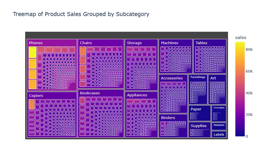
- Total sales of all subcategories
- Category Gross Margin
- Sales in each market for each country
- Sales of each category in each market
- Cumulative sales of each category based on time
- Sales based on week number
- Shipments mode based on sub-category
- Sales for state and city
- Sales per week and staffing needs per week
Category Distribution#
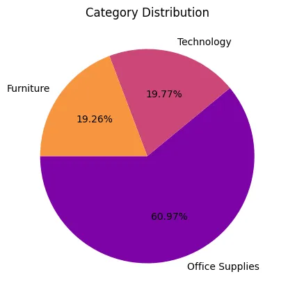
We find out that most of our sales are office supplies.
Click on each subcategory to see the sales and products of that subcategory. Click the top bar to go back to the main view.
Category Overview#
Click on each subcategory to see the sales and products of that subcategory. Click again to go back to the main view.
We can very well see the subcategories of our products.
Customer Lifetime Value#
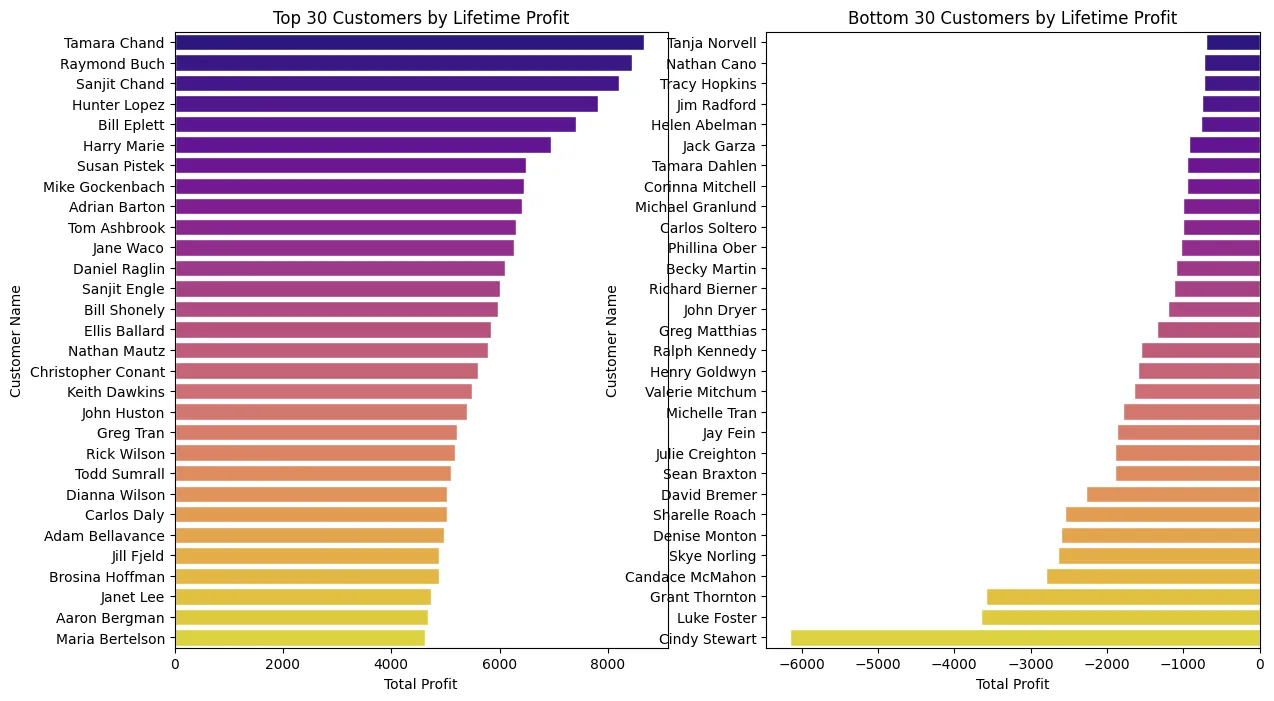
We can see our most profitable and least profitable customers together. We seem to have a customer named Cindy Steward that has a very negative amount of profit. Lets investigate further.
Case Study: Visualizing Cindy Steward#
Cindy Stewart is the most unprofitable customer found. We should find who Cindy Stewart is and how she was able to make so much money just buying stuff from this company, leading to us losing so much money.
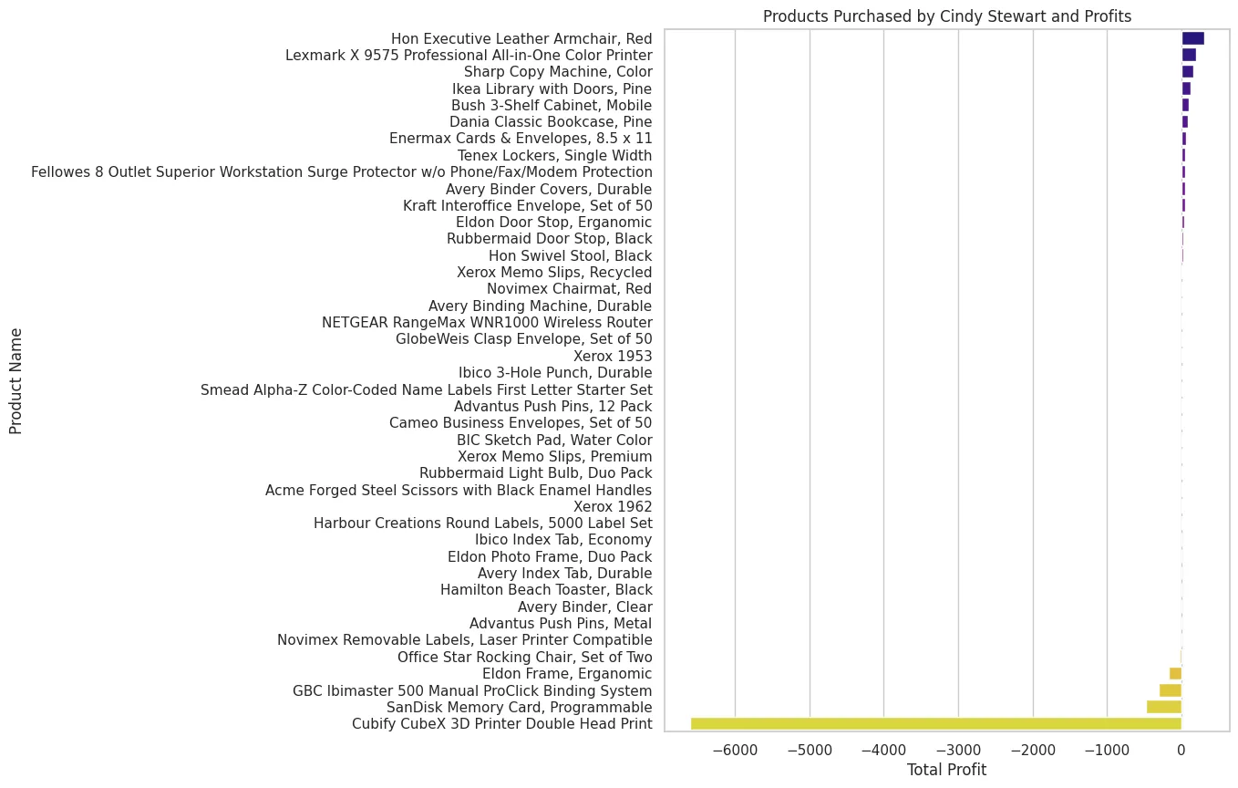
It turns out it we should stop selling the cubify CubeX and sandisk memory products and we would be so much less unprofitable.
Sales of each subcategory#
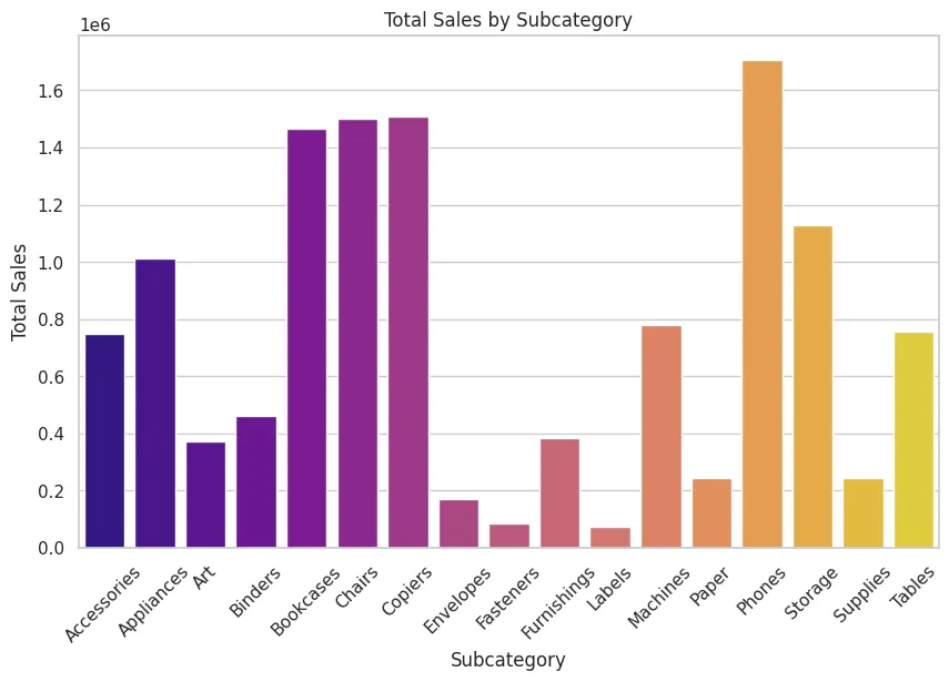
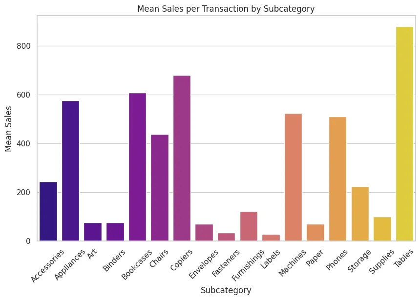
We see that the store is selling way too many tables. Probably because the price is way too cheap and unprofitable for us (and profitable for customers) as we are going to find out later.
Sales in each market#
Sales in each market#
Part 4- Conclusions#
By utilizing pandas, python and plotting libraries like matplotlib, seaborn and plotly we learned.
- High discounts correlate with more unprofitable sales.
- Technology category leads in profitability, while Furniture often shows lower margins.
- United States dominates in total sales, canada is the best market for expansion.
- Many many states are overall unprofitable. we should really address this. maybe close the worst branches.
- Standard shipping class is the most used shipping.
- Subcategories like Copiers and Phones are consistently profitable, making them strategic focus areas.
- We should stop selling tables or agressively increase prices.
- Some items like CubeX are unprofitable. We should address these items.